Introduction to tmtyro
Simplified workflows for text-mining tyros
Source:vignettes/articles/tmtyro.Rmd
tmtyro.RmdWorking with text as data is a multi-step process. After choosing and collecting documents, you’ll need to load them in some structured way before anything else. Only then is it possible to “do” text analysis: tagging parts of speech, normalizing by lemma, comparing features, measuring sentiment, and so on. Even then, you’ll need to communicate findings by preparing compelling explanations, tables, and visualizations of your results.
The tmtyro package aims to make these steps fast and easy.
- Purpose-built functions for collecting a corpus let you focus on what instead of how.
- Scalable functions for loading a corpus provide room for growth, from simple word count to grammar parsing and lemmatizing.
- Additional functions standardize approaches for measuring word use and vocabulary uniqueness, detecting sentiment, assessing term frequency–inverse document frequency, working with n-grams, and even building topic models.
- One simple function prepares publication-ready tables, automatically adjusting based on the kind of data used. Another simple function prepares compelling visualizations, returning clean, publication-ready figures.
- When it’s time to share your work, a function prepares a narrative of the process that was automatically logged along the way.
- Every step is offered as a verb using complementary syntax. This keeps workflows easy to build, easy to understand, easy to explain, and easy to reproduce.
Preparing texts
tmtyro offers a few functions to gather and load texts for study:
-
get_gutenberg_corpus()caches the HTML version of books by their Project Gutenberg ID, parses their text and headers, and presents them in a table. -
get_micusp_corpus()caches papers from the Michigan Corpus of Upper-level Student Papers, parses them for metadata and contents, and presents them in a table. -
download_once()caches an online file and passes the local path invisibly. -
load_texts()prepares a table in “tidytext” format with one word per row and columns for metadata. These texts can be loaded from a folder of files or passed from a table. Parameters allow for lemmatization, part-of-speech processing, and other options.
Other functions aid with preparing a corpus:
-
move_header_to_text()corrects overzealous identification of HTML headers when parsing books from Project Gutenberg. -
standardize_titles()converts a vector or column into title case, converts underscores with spaces, and optionally removes initial articles. -
identify_by()sets a column of metadata to serve as document marker.
Get a corpus
Collecting texts from Project Gutenberg will be a common first step
for many. The function get_gutenberg_corpus() needs only
the Gutenberg ID number, found in the book’s URL. The resulting table
draws metadata from the gutenbergr package, with columns for
“gutenberg_id”, “title”, “author”, headers such as those used for
chapters, and “text.”
library(tmtyro)
joyce <- get_gutenberg_corpus(c(2814, 4217, 4300))

joyce
#> # A tibble: 10,810 × 7
#>    gutenberg_id title     author       part        section subsection text
#>           <int> <chr>     <chr>        <chr>       <chr>   <chr>      <chr>
#>  1         2814 Dubliners Joyce, James THE SISTERS NA      NA         There was…
#>  2         2814 Dubliners Joyce, James THE SISTERS NA      NA         Old Cotte…
#>  3         2814 Dubliners Joyce, James THE SISTERS NA      NA         “No, I wo…
#>  4         2814 Dubliners Joyce, James THE SISTERS NA      NA         He began …
#>  5         2814 Dubliners Joyce, James THE SISTERS NA      NA         “I have m…
#>  6         2814 Dubliners Joyce, James THE SISTERS NA      NA         He began …
#>  7         2814 Dubliners Joyce, James THE SISTERS NA      NA         “Well, so…
#>  8         2814 Dubliners Joyce, James THE SISTERS NA      NA         “Who?” sa…
#>  9         2814 Dubliners Joyce, James THE SISTERS NA      NA         “Father F…
#> 10         2814 Dubliners Joyce, James THE SISTERS NA      NA         “Is he de…
#> # ℹ 10,800 more rows
In some cases, headers may make better sense if read as part of the text, as in the “Aeolus” chapter of Ulysses, where frequent newspaper headlines pepper the page:
ulysses <- get_gutenberg_corpus(4300)

# dplyr is used here to choose a smaller example for comparison
ulysses |>
  dplyr::filter(section == "[ 7 ]")
#> # A tibble: 476 × 7
#>    gutenberg_id title   author       part   section subsection             text
#>           <int> <chr>   <chr>        <chr>  <chr>   <chr>                  <chr>
#>  1         4300 Ulysses Joyce, James — II — [ 7 ]   IN THE HEART OF THE H… Befo…
#>  2         4300 Ulysses Joyce, James — II — [ 7 ]   IN THE HEART OF THE H… —Rat…
#>  3         4300 Ulysses Joyce, James — II — [ 7 ]   IN THE HEART OF THE H… —Com…
#>  4         4300 Ulysses Joyce, James — II — [ 7 ]   IN THE HEART OF THE H… Righ…
#>  5         4300 Ulysses Joyce, James — II — [ 7 ]   IN THE HEART OF THE H… —Sta…
#>  6         4300 Ulysses Joyce, James — II — [ 7 ]   THE WEARER OF THE CRO… Unde…
#>  7         4300 Ulysses Joyce, James — II — [ 7 ]   GENTLEMEN OF THE PRESS Gros…
#>  8         4300 Ulysses Joyce, James — II — [ 7 ]   GENTLEMEN OF THE PRESS —The…
#>  9         4300 Ulysses Joyce, James — II — [ 7 ]   GENTLEMEN OF THE PRESS —Jus…
#> 10         4300 Ulysses Joyce, James — II — [ 7 ]   GENTLEMEN OF THE PRESS The …
#> # ℹ 466 more rows
These can be corrected with move_header_to_text().
ulysses <- get_gutenberg_corpus(4300) |>
  move_header_to_text(subsection)

# dplyr is used here to choose a smaller example for comparison
ulysses |>
  dplyr::filter(section == "[ 7 ]")
#> # A tibble: 539 × 6
#>    gutenberg_id title   author       part   section text
#>           <int> <chr>   <chr>        <chr>  <chr>   <chr>
#>  1         4300 Ulysses Joyce, James — II — [ 7 ]   IN THE HEART OF THE HIBERNI…
#>  2         4300 Ulysses Joyce, James — II — [ 7 ]   Before Nelson’s pillar tram…
#>  3         4300 Ulysses Joyce, James — II — [ 7 ]   —Rathgar and Terenure!
#>  4         4300 Ulysses Joyce, James — II — [ 7 ]   —Come on, Sandymount Green!
#>  5         4300 Ulysses Joyce, James — II — [ 7 ]   Right and left parallel cla…
#>  6         4300 Ulysses Joyce, James — II — [ 7 ]   —Start, Palmerston Park!
#>  7         4300 Ulysses Joyce, James — II — [ 7 ]   THE WEARER OF THE CROWN
#>  8         4300 Ulysses Joyce, James — II — [ 7 ]   Under the porch of the gene…
#>  9         4300 Ulysses Joyce, James — II — [ 7 ]   GENTLEMEN OF THE PRESS
#> 10         4300 Ulysses Joyce, James — II — [ 7 ]   Grossbooted draymen rolled …
#> # ℹ 529 more rows
Headers can be moved for specific texts in a corpus by specifying a
filter like title == "Ulysses":
joyce <- joyce |>
  move_header_to_text(subsection, title == "Ulysses")

joyce |>
  dplyr::filter(section == "[ 7 ]")
#> # A tibble: 539 × 6
#>    gutenberg_id title   author       part   section text
#>           <int> <chr>   <chr>        <chr>  <chr>   <chr>
#>  1         4300 Ulysses Joyce, James — II — [ 7 ]   IN THE HEART OF THE HIBERNI…
#>  2         4300 Ulysses Joyce, James — II — [ 7 ]   Before Nelson’s pillar tram…
#>  3         4300 Ulysses Joyce, James — II — [ 7 ]   —Rathgar and Terenure!
#>  4         4300 Ulysses Joyce, James — II — [ 7 ]   —Come on, Sandymount Green!
#>  5         4300 Ulysses Joyce, James — II — [ 7 ]   Right and left parallel cla…
#>  6         4300 Ulysses Joyce, James — II — [ 7 ]   —Start, Palmerston Park!
#>  7         4300 Ulysses Joyce, James — II — [ 7 ]   THE WEARER OF THE CROWN
#>  8         4300 Ulysses Joyce, James — II — [ 7 ]   Under the porch of the gene…
#>  9         4300 Ulysses Joyce, James — II — [ 7 ]   GENTLEMEN OF THE PRESS
#> 10         4300 Ulysses Joyce, James — II — [ 7 ]   Grossbooted draymen rolled …
#> # ℹ 529 more rows
Load texts
load_texts() prepares a set of documents for study,
either from a table or from a folder of files.
From a table
A table like the one prepared by get_gutenberg_corpus()
can be prepared in tidytext format with one word per row using
load_texts().
corpus_ulysses <- ulysses |>
  load_texts()

corpus_ulysses
#> # A tibble: 265,043 × 6
#>    doc_id title   author       part  section word
#>     <int> <chr>   <chr>        <chr> <chr>   <chr>
#>  1   4300 Ulysses Joyce, James — I — [ 1 ]   stately
#>  2   4300 Ulysses Joyce, James — I — [ 1 ]   plump
#>  3   4300 Ulysses Joyce, James — I — [ 1 ]   buck
#>  4   4300 Ulysses Joyce, James — I — [ 1 ]   mulligan
#>  5   4300 Ulysses Joyce, James — I — [ 1 ]   came
#>  6   4300 Ulysses Joyce, James — I — [ 1 ]   from
#>  7   4300 Ulysses Joyce, James — I — [ 1 ]   the
#>  8   4300 Ulysses Joyce, James — I — [ 1 ]   stairhead
#>  9   4300 Ulysses Joyce, James — I — [ 1 ]   bearing
#> 10   4300 Ulysses Joyce, James — I — [ 1 ]   a
#> # ℹ 265,033 more rows
From files
If text files are already collected in a folder on disk, they can be
prepared in a table by passing the path to the folder inside
load_texts(). Used this way, load_texts() will
load up every file using the “txt” file extension, populating the
doc_id column with the first part of the file name.
corpus_austen <- load_texts("austen")In this example, the “austen” folder is found within the current
project. If it was instead found somewhere else on the computer, the
complete path can be passed like this:load_texts("~/corpora/austen")
Choose a different doc_id
Documents loaded from get_gutenberg_corpus() use the
gutenberg_id column as their document identifier.
corpus_dubliners <- get_gutenberg_corpus(2814) |>
  load_texts(lemma = TRUE, pos = TRUE)

corpus_dubliners
#> # A tibble: 67,885 × 7
#>    doc_id title     author       part        word  pos   lemma
#>     <int> <chr>     <chr>        <chr>       <chr> <chr> <chr>
#>  1   2814 Dubliners Joyce, James THE SISTERS there EX    there
#>  2   2814 Dubliners Joyce, James THE SISTERS was   VBD   be
#>  3   2814 Dubliners Joyce, James THE SISTERS no    DT    no
#>  4   2814 Dubliners Joyce, James THE SISTERS hope  NN    hope
#>  5   2814 Dubliners Joyce, James THE SISTERS for   IN    for
#>  6   2814 Dubliners Joyce, James THE SISTERS him   PRP   him
#>  7   2814 Dubliners Joyce, James THE SISTERS this  DT    this
#>  8   2814 Dubliners Joyce, James THE SISTERS time  NN    time
#>  9   2814 Dubliners Joyce, James THE SISTERS it    PRP   it
#> 10   2814 Dubliners Joyce, James THE SISTERS was   VBD   be
#> # ℹ 67,875 more rows
If a different column is preferred, identify_by() makes
the switch. In this example from Dubliners, for instance, each
story’s title is shown under “part”. identify_by() makes it
easy to identify documents by that column:
corpus_dubliners <- corpus_dubliners |>
  identify_by(part)

corpus_dubliners
#> # A tibble: 67,885 × 7
#>    doc_id      title     author       part        word  pos   lemma
#>    <fct>       <chr>     <chr>        <chr>       <chr> <chr> <chr>
#>  1 THE SISTERS Dubliners Joyce, James THE SISTERS there EX    there
#>  2 THE SISTERS Dubliners Joyce, James THE SISTERS was   VBD   be
#>  3 THE SISTERS Dubliners Joyce, James THE SISTERS no    DT    no
#>  4 THE SISTERS Dubliners Joyce, James THE SISTERS hope  NN    hope
#>  5 THE SISTERS Dubliners Joyce, James THE SISTERS for   IN    for
#>  6 THE SISTERS Dubliners Joyce, James THE SISTERS him   PRP   him
#>  7 THE SISTERS Dubliners Joyce, James THE SISTERS this  DT    this
#>  8 THE SISTERS Dubliners Joyce, James THE SISTERS time  NN    time
#>  9 THE SISTERS Dubliners Joyce, James THE SISTERS it    PRP   it
#> 10 THE SISTERS Dubliners Joyce, James THE SISTERS was   VBD   be
#> # ℹ 67,875 more rows
Standardize titles
standardize_titles() converts titles to something
cleaner by adopting title case.
before <- unique(corpus_dubliners$doc_id)

corpus_dubliners <- corpus_dubliners |>
  standardize_titles()

after <- unique(corpus_dubliners$doc_id)

data.frame(before, after)
#>                           before                         after
#> 1                    THE SISTERS                   The Sisters
#> 2                   AN ENCOUNTER                  An Encounter
#> 3                          ARABY                         Araby
#> 4                        EVELINE                       Eveline
#> 5                 AFTER THE RACE                After the Race
#> 6                   TWO GALLANTS                  Two Gallants
#> 7             THE BOARDING HOUSE            The Boarding House
#> 8                 A LITTLE CLOUD                A Little Cloud
#> 9                   COUNTERPARTS                  Counterparts
#> 10                          CLAY                          Clay
#> 11                A PAINFUL CASE                A Painful Case
#> 12 IVY DAY IN THE COMMITTEE ROOM Ivy Day in the Committee Room
#> 13                      A MOTHER                      A Mother
#> 14                         GRACE                         Grace
#> 15                      THE DEAD                      The Dead
Studying texts
Useful at many stages of work with a corpus,
contextualize() shows the context of a search term, with an
adjustable window on either side and options for searching with regular
expressions. Most other functions for studying texts follow a
predictable naming convention:
-
add_frequency()adds a column for word frequencies. -
add_vocabulary()adds columns measuring the lexical variety of texts. -
add_sentiment()adds a column of sentiment identifiers from a chosen lexicon. -
add_ngrams()adds columns of words for bigrams, trigrams, or more.
Not every method preserves the size or shape of data passed to it:
-
summarize_tf_idf()returns a data frame for every unique token in each document in a corpus, with columns indicating weights for term frequency-inverse document frequency.
Along with these, other functions assist with the process:
-
drop_na()drops rows with missing data in any column or in specified columns. -
combine_ngrams()combines multiple columns for n-grams into one. -
separate_ngrams()separatesa single column of n-grams into one column per word.
But understanding context of key words with
contextualize() might be especially helpful.
Showing context
contextualize() finds uses of a word within a corpus and
returns a window of context around each use.
corpus_dubliners |>
  contextualize("snow")
#> mat scraping the snow from his goloshes
#> light fringe of snow lay like a
#> home in the snow if she were
#> the park the snow would be lying
#> standing in the snow on the quay
By default, contextualize() returns five results,
showing a window of three words before and after an exact search term.
Adjusting limit changes the number of results, with
limit = 0 returning a table. Other options include
window to adjust the number of words shown and
regex to accept partial matches.
corpus_dubliners |>
  contextualize(regex = "sno",
                window = 2,
                limit = 0)
#> # A tibble: 22 × 4
#>    doc_id         word           index context
#>    <fct>          <chr>          <int> <chr>
#>  1 After the Race snorting        1088 to the SNOrting motor the
#>  2 The Dead       snow             610 scraping the SNOw from his
#>  3 The Dead       snow             705 fringe of SNOw lay like
#>  4 The Dead       snow_stiffened   739 through the SNOw_stiffened frieze a
#>  5 The Dead       snowing          754 is it SNOwing again mr
#>  6 The Dead       snow            1660 in the SNOw if she
#>  7 The Dead       snow            5411 park the SNOw would be
#>  8 The Dead       snow            8739 in the SNOw on the
#>  9 The Dead       snow            8773 weighted with SNOw the wellington
#> 10 The Dead       snow            8782 cap of SNOw that flashed
#> # ℹ 12 more rows
When loading texts, load_texts() provides an option to
keep original capitalization and punctuation. This option doesn’t always
work, and it seems incompatible with the current implementation of
part-of-speech parsing, so it’s not always appropriate. But using
contextualize() on corpora loaded with
load_texts(keep_original = TRUE) will show search terms
much closer to their original context:
corpus_joyce <- joyce |>
  load_texts(keep_original = TRUE) |>
  identify_by(title)

tundish <-
  corpus_joyce |>
  contextualize("tundish", limit = 1:7)
#> it not a tundish? —What is a
#> —What is a tundish? —That. The the
#> that called a tundish in Ireland? asked
#> is called a tundish in Lower Drumcondra,
#> best English. —A tundish, said the dean
#> word yet again. —Tundish! Well now, that
#> April 13. That tundish has been on
Even when limit is set to some value other than 0, the
table of results is returned invisibly for later recall.
tundish
#> # A tibble: 7 × 4
#>   doc_id                                  word    index context
#>   <fct>                                   <chr>   <int> <chr>
#> 1 A Portrait of the Artist as a Young Man tundish 63827 it not a TUNDISH? —What…
#> 2 A Portrait of the Artist as a Young Man tundish 63831 —What is a TUNDISH? —Th…
#> 3 A Portrait of the Artist as a Young Man tundish 63840 that called a TUNDISH i…
#> 4 A Portrait of the Artist as a Young Man tundish 63858 is called a TUNDISH in …
#> 5 A Portrait of the Artist as a Young Man tundish 63872 best English. —A TUNDIS…
#> 6 A Portrait of the Artist as a Young Man tundish 64122 word yet again. —TUNDIS…
#> 7 A Portrait of the Artist as a Young Man tundish 84352 April 13. That TUNDISH …
Word frequencies
add_frequency() adds word counts for each document in a
new column, n.
counts_dubliners <-
  corpus_dubliners |>
  add_frequency()

counts_dubliners
#> # A tibble: 67,885 × 8
#>    doc_id      title     author       part        word  pos   lemma     n
#>    <fct>       <chr>     <chr>        <chr>       <chr> <chr> <chr> <int>
#>  1 The Sisters Dubliners Joyce, James THE SISTERS there EX    there    15
#>  2 The Sisters Dubliners Joyce, James THE SISTERS was   VBD   be       57
#>  3 The Sisters Dubliners Joyce, James THE SISTERS no    DT    no       16
#>  4 The Sisters Dubliners Joyce, James THE SISTERS hope  NN    hope      1
#>  5 The Sisters Dubliners Joyce, James THE SISTERS for   IN    for      32
#>  6 The Sisters Dubliners Joyce, James THE SISTERS him   PRP   him      43
#>  7 The Sisters Dubliners Joyce, James THE SISTERS this  DT    this      6
#>  8 The Sisters Dubliners Joyce, James THE SISTERS time  NN    time      3
#>  9 The Sisters Dubliners Joyce, James THE SISTERS it    PRP   it       40
#> 10 The Sisters Dubliners Joyce, James THE SISTERS was   VBD   be       57
#> # ℹ 67,875 more rows
To count by some other column, indicate it in the parentheses:
corpus_dubliners |>
  add_frequency(lemma)
#> # A tibble: 67,885 × 8
#>    doc_id      title     author       part        word  pos   lemma     n
#>    <fct>       <chr>     <chr>        <chr>       <chr> <chr> <chr> <int>
#>  1 The Sisters Dubliners Joyce, James THE SISTERS there EX    there    15
#>  2 The Sisters Dubliners Joyce, James THE SISTERS was   VBD   be       98
#>  3 The Sisters Dubliners Joyce, James THE SISTERS no    DT    no       16
#>  4 The Sisters Dubliners Joyce, James THE SISTERS hope  NN    hope      1
#>  5 The Sisters Dubliners Joyce, James THE SISTERS for   IN    for      32
#>  6 The Sisters Dubliners Joyce, James THE SISTERS him   PRP   him      43
#>  7 The Sisters Dubliners Joyce, James THE SISTERS this  DT    this      9
#>  8 The Sisters Dubliners Joyce, James THE SISTERS time  NN    time      3
#>  9 The Sisters Dubliners Joyce, James THE SISTERS it    PRP   it       40
#> 10 The Sisters Dubliners Joyce, James THE SISTERS was   VBD   be       98
#> # ℹ 67,875 more rows
Document-frequency matrix
Alternatively, word frequencies can be shown in a document-frequency
matrix using expand_documents():
corpus_dubliners |>
  expand_documents()
#> # A tibble: 15 × 7,505
#>    doc_id         the    and     of     to      he      a     was     his   `in`
#>    <fct>        <dbl>  <dbl>  <dbl>  <dbl>   <dbl>  <dbl>   <dbl>   <dbl>  <dbl>
#>  1 The Sisters 0.0551 0.0380 0.0222 0.0303 0.0180  0.0148 0.0184  0.0158  0.0174
#>  2 An Encount… 0.0557 0.0329 0.0274 0.0265 0.0311  0.0219 0.0182  0.0108  0.0129
#>  3 Araby       0.0815 0.0300 0.0275 0.0300 0.00686 0.0210 0.0172  0.00343 0.0176
#>  4 Eveline     0.0563 0.0252 0.0257 0.0372 0.0246  0.0219 0.0224  0.00601 0.0180
#>  5 After the … 0.0729 0.0300 0.0447 0.0251 0.0197  0.0300 0.0268  0.0183  0.0215
#>  6 Two Gallan… 0.0550 0.0333 0.0333 0.0241 0.0417  0.0289 0.0143  0.0287  0.0120
#>  7 The Boardi… 0.0498 0.0319 0.0316 0.0316 0.0244  0.0276 0.0215  0.0176  0.0133
#>  8 A Little C… 0.0502 0.0356 0.0263 0.0247 0.0346  0.0204 0.0138  0.0261  0.0146
#>  9 Counterpar… 0.0763 0.0329 0.0276 0.0266 0.0337  0.0229 0.0188  0.0237  0.0163
#> 10 Clay        0.0597 0.0529 0.0230 0.0302 0.00982 0.0204 0.0272  0.00415 0.0117
#> 11 A Painful … 0.0668 0.0268 0.0353 0.0276 0.0400  0.0257 0.0138  0.0251  0.0191
#> 12 Ivy Day in… 0.0610 0.0242 0.0232 0.0212 0.0259  0.0274 0.00762 0.0160  0.0128
#> 13 A Mother    0.0619 0.0349 0.0228 0.0305 0.0170  0.0212 0.0230  0.0108  0.0153
#> 14 Grace       0.0644 0.0268 0.0300 0.0224 0.0235  0.0258 0.0179  0.0190  0.0150
#> 15 The Dead    0.0553 0.0364 0.0252 0.0234 0.0181  0.0217 0.0160  0.0160  0.0167
#> # ℹ 7,495 more variables: her <dbl>, had <dbl>, said <dbl>, that <dbl>,
#> #   it <dbl>, with <dbl>, `for` <dbl>, him <dbl>, at <dbl>, on <dbl>, i <dbl>,
#> #   she <dbl>, but <dbl>, as <dbl>, were <dbl>, when <dbl>, all <dbl>,
#> #   you <dbl>, would <dbl>, they <dbl>, not <dbl>, out <dbl>, be <dbl>,
#> #   up <dbl>, by <dbl>, one <dbl>, from <dbl>, an <dbl>, then <dbl>,
#> #   little <dbl>, what <dbl>, no <dbl>, have <dbl>, there <dbl>, them <dbl>,
#> #   which <dbl>, so <dbl>, could <dbl>, `if` <dbl>, into <dbl>, went <dbl>, …
Vocabulary richness
add_vocabulary() adds measurements of vocabulary
richness, including cumulative vocabulary size and indicators of hapax
legomena.
vocab_dubliners <-
  corpus_dubliners |>
  add_vocabulary()

vocab_dubliners
#> # A tibble: 67,885 × 13
#>    doc_id   title author part  word  pos   lemma new_word hapax_doc hapax_corpus
#>    <fct>    <chr> <chr>  <chr> <chr> <chr> <chr> <lgl>    <lgl>     <lgl>
#>  1 The Sis… Dubl… Joyce… THE … there EX    there TRUE     FALSE     FALSE
#>  2 The Sis… Dubl… Joyce… THE … was   VBD   be    TRUE     FALSE     FALSE
#>  3 The Sis… Dubl… Joyce… THE … no    DT    no    TRUE     FALSE     FALSE
#>  4 The Sis… Dubl… Joyce… THE … hope  NN    hope  TRUE     TRUE      FALSE
#>  5 The Sis… Dubl… Joyce… THE … for   IN    for   TRUE     FALSE     FALSE
#>  6 The Sis… Dubl… Joyce… THE … him   PRP   him   TRUE     FALSE     FALSE
#>  7 The Sis… Dubl… Joyce… THE … this  DT    this  TRUE     FALSE     FALSE
#>  8 The Sis… Dubl… Joyce… THE … time  NN    time  TRUE     FALSE     FALSE
#>  9 The Sis… Dubl… Joyce… THE … it    PRP   it    TRUE     FALSE     FALSE
#> 10 The Sis… Dubl… Joyce… THE … was   VBD   be    FALSE    FALSE     FALSE
#> # ℹ 67,875 more rows
#> # ℹ 3 more variables: vocabulary <int>, ttr <dbl>, hir <dbl>
Sentiment
add_sentiment() adds measurements of sentiment using the
“Bing” lexicon by default.
sentiment_dubliners <- corpus_dubliners |>
  add_sentiment()

sentiment_dubliners
#> # A tibble: 67,886 × 8
#> doc_id title author part word pos lemma sentiment
#> <fct> <chr> <chr> <chr> <chr> <chr> <chr> <chr>
#> 1 The Sisters Dubliners Joyce, James THE SISTERS there EX there NA
#> 2 The Sisters Dubliners Joyce, James THE SISTERS was VBD be NA
#> 3 The Sisters Dubliners Joyce, James THE SISTERS no DT no NA
#> 4 The Sisters Dubliners Joyce, James THE SISTERS hope NN hope NA
#> 5 The Sisters Dubliners Joyce, James THE SISTERS for IN for NA
#> 6 The Sisters Dubliners Joyce, James THE SISTERS him PRP him NA
#> 7 The Sisters Dubliners Joyce, James THE SISTERS this DT this NA
#> 8 The Sisters Dubliners Joyce, James THE SISTERS time NN time NA
#> 9 The Sisters Dubliners Joyce, James THE SISTERS it PRP it NA
#> 10 The Sisters Dubliners Joyce, James THE SISTERS was VBD be NA
#> # ℹ 67,876 more rowsDropping empty rows
Since many words may not be found in a given sentiment lexicon,
drop_na() makes it easy to remove empty rows.
sentiment_dubliners |>
  drop_na(sentiment)
#> # A tibble: 3,787 × 8
#>    doc_id      title     author       part        word     pos   lemma sentiment
#>    <fct>       <chr>     <chr>        <chr>       <chr>    <chr> <chr> <chr>
#>  1 The Sisters Dubliners Joyce, James THE SISTERS evenly   RB    even… positive
#>  2 The Sisters Dubliners Joyce, James THE SISTERS dead     JJ    dead  negative
#>  3 The Sisters Dubliners Joyce, James THE SISTERS darkened VBN   dark… negative
#>  4 The Sisters Dubliners Joyce, James THE SISTERS blind    NN    blind negative
#>  5 The Sisters Dubliners Joyce, James THE SISTERS idle     VB    idle  negative
#>  6 The Sisters Dubliners Joyce, James THE SISTERS strange… RB    stra… negative
#>  7 The Sisters Dubliners Joyce, James THE SISTERS like     IN    like  positive
#>  8 The Sisters Dubliners Joyce, James THE SISTERS like     IN    like  positive
#>  9 The Sisters Dubliners Joyce, James THE SISTERS sinful   JJ    sinf… negative
#> 10 The Sisters Dubliners Joyce, James THE SISTERS fear     NN    fear  negative
#> # ℹ 3,777 more rows
Choosing a sentiment lexicon
The lexicon can be chosen at measurement.
sentiment_ulysses <- ulysses |>
  load_texts() |>
  identify_by(section) |>
  add_sentiment(lexicon = "nrc")

sentiment_ulysses |>
  drop_na(sentiment)
#> # A tibble: 63,006 × 7
#> doc_id title author part section word sentiment
#> <fct> <chr> <chr> <chr> <chr> <chr> <chr>
#> 1 [ 1 ] Ulysses Joyce, James — I — [ 1 ] stately positive
#> 2 [ 1 ] Ulysses Joyce, James — I — [ 1 ] plump anticipation
#> 3 [ 1 ] Ulysses Joyce, James — I — [ 1 ] buck fear
#> 4 [ 1 ] Ulysses Joyce, James — I — [ 1 ] buck negative
#> 5 [ 1 ] Ulysses Joyce, James — I — [ 1 ] buck positive
#> 6 [ 1 ] Ulysses Joyce, James — I — [ 1 ] buck surprise
#> 7 [ 1 ] Ulysses Joyce, James — I — [ 1 ] razor fear
#> 8 [ 1 ] Ulysses Joyce, James — I — [ 1 ] dark sadness
#> 9 [ 1 ] Ulysses Joyce, James — I — [ 1 ] fearful fear
#> 10 [ 1 ] Ulysses Joyce, James — I — [ 1 ] fearful negative
#> # ℹ 62,996 more rowsN-grams
Following the same pattern, add_ngrams() adds columns
for n-length phrases of words. By default, it prepares bigrams (or
2-grams).
bigrams_joyce <- corpus_joyce |>
  add_ngrams()

bigrams_joyce
#> # A tibble: 417,846 × 8
#>    doc_id    title     author       part        section original word_1 word_2
#>    <fct>     <chr>     <chr>        <chr>       <chr>   <chr>    <chr>  <chr>
#>  1 Dubliners Dubliners Joyce, James THE SISTERS NA      There    there  was
#>  2 Dubliners Dubliners Joyce, James THE SISTERS NA      was      was    no
#>  3 Dubliners Dubliners Joyce, James THE SISTERS NA      no       no     hope
#>  4 Dubliners Dubliners Joyce, James THE SISTERS NA      hope     hope   for
#>  5 Dubliners Dubliners Joyce, James THE SISTERS NA      for      for    him
#>  6 Dubliners Dubliners Joyce, James THE SISTERS NA      him      him    this
#>  7 Dubliners Dubliners Joyce, James THE SISTERS NA      this     this   time
#>  8 Dubliners Dubliners Joyce, James THE SISTERS NA      time:    time   it
#>  9 Dubliners Dubliners Joyce, James THE SISTERS NA      it       it     was
#> 10 Dubliners Dubliners Joyce, James THE SISTERS NA      was      was    the
#> # ℹ 417,836 more rows
Other n-grams can be chosen by passing a vector of numbers.
trigrams_joyce <- corpus_joyce |>
  add_ngrams(1:3)

trigrams_joyce
#> # A tibble: 417,846 × 9
#>    doc_id    title     author       part   section original word_1 word_2 word_3
#>    <fct>     <chr>     <chr>        <chr>  <chr>   <chr>    <chr>  <chr>  <chr>
#>  1 Dubliners Dubliners Joyce, James THE S… NA      There    there  was    no
#>  2 Dubliners Dubliners Joyce, James THE S… NA      was      was    no     hope
#>  3 Dubliners Dubliners Joyce, James THE S… NA      no       no     hope   for
#>  4 Dubliners Dubliners Joyce, James THE S… NA      hope     hope   for    him
#>  5 Dubliners Dubliners Joyce, James THE S… NA      for      for    him    this
#>  6 Dubliners Dubliners Joyce, James THE S… NA      him      him    this   time
#>  7 Dubliners Dubliners Joyce, James THE S… NA      this     this   time   it
#>  8 Dubliners Dubliners Joyce, James THE S… NA      time:    time   it     was
#>  9 Dubliners Dubliners Joyce, James THE S… NA      it       it     was    the
#> 10 Dubliners Dubliners Joyce, James THE S… NA      was      was    the    third
#> # ℹ 417,836 more rows
Tf-idf
add_tf_idf() adds measurements of term frequency
(tf), inverse document frequency (idf), and
combined term frequency–inverse document frequency
(tf_idf).
corpus_dubliners |>
  add_tf_idf()
#> # A tibble: 67,885 × 11
#>    doc_id      title author part  word  pos   lemma     n      tf    idf  tf_idf
#>    <fct>       <chr> <chr>  <chr> <chr> <chr> <chr> <int>   <dbl>  <dbl>   <dbl>
#>  1 The Sisters Dubl… Joyce… THE … there EX    there    15 0.0048  0      0
#>  2 The Sisters Dubl… Joyce… THE … was   VBD   be       57 0.0182  0      0
#>  3 The Sisters Dubl… Joyce… THE … no    DT    no       16 0.00512 0      0
#>  4 The Sisters Dubl… Joyce… THE … hope  NN    hope      1 0.00032 0.511  1.63e-4
#>  5 The Sisters Dubl… Joyce… THE … for   IN    for      32 0.0102  0      0
#>  6 The Sisters Dubl… Joyce… THE … him   PRP   him      43 0.0138  0      0
#>  7 The Sisters Dubl… Joyce… THE … this  DT    this      6 0.00192 0.0690 1.32e-4
#>  8 The Sisters Dubl… Joyce… THE … time  NN    time      3 0.00096 0      0
#>  9 The Sisters Dubl… Joyce… THE … it    PRP   it       40 0.0128  0      0
#> 10 The Sisters Dubl… Joyce… THE … was   VBD   be       57 0.0182  0      0
#> # ℹ 67,875 more rows
Term frequency–inverse document frequency is most commonly used as a
way of summarizing language used, paying less attention word order and
reducing documents to one instance of each token. To study texts this
way, summarize_tf_idf() returns a table arranged in
descending strength of tf-idf.
tfidf_dubliners <- corpus_dubliners |>
  summarize_tf_idf()

tfidf_dubliners
#> # A tibble: 17,656 × 6
#>    doc_id                        word         n      tf   idf tf_idf
#>    <fct>                         <chr>    <int>   <dbl> <dbl>  <dbl>
#>  1 Clay                          maria       40 0.0151   2.71 0.0409
#>  2 Two Gallants                  corley      46 0.0117   2.71 0.0318
#>  3 After the Race                jimmy       24 0.0107   2.71 0.0291
#>  4 Ivy Day in the Committee Room henchy      53 0.0101   2.71 0.0272
#>  5 A Little Cloud                gallaher    48 0.00964  2.71 0.0261
#>  6 The Dead                      gabriel    142 0.00906  2.71 0.0245
#>  7 Grace                         kernan      66 0.00873  2.71 0.0236
#>  8 Ivy Day in the Committee Room o’connor    45 0.00854  2.71 0.0231
#>  9 A Little Cloud                chandler    41 0.00823  2.71 0.0223
#> 10 A Mother                      kearney     50 0.0110   2.01 0.0223
#> # ℹ 17,646 more rows
Tf-idf’s method understandably emphasizes proper nouns that are
unique to each document. The remove_names argument in
load_texts() can help to filter out words that appear only
in capitalized form. Removing names from Dubliners makes a
noticeable difference in tf-idf results:
tfidf_dubliners <- get_gutenberg_corpus(2814) |>
  load_texts(remove_names = TRUE) |>
  identify_by(part) |>
  standardize_titles() |>
  summarize_tf_idf()

tfidf_dubliners
#> # A tibble: 16,721 × 6
#>    doc_id         word         n      tf   idf  tf_idf
#>    <fct>          <chr>    <int>   <dbl> <dbl>   <dbl>
#>  1 The Dead       aunt       101 0.00693 1.61  0.0112
#>  2 Araby          bazaar       9 0.00406 2.71  0.0110
#>  3 The Sisters    aunt        19 0.00649 1.61  0.0104
#>  4 After the Race cars         6 0.00286 2.71  0.00773
#>  5 An Encounter   we          58 0.0189  0.405 0.00767
#>  6 After the Race car         11 0.00524 1.32  0.00692
#>  7 Eveline        avenue       4 0.00225 2.71  0.00610
#>  8 Counterparts   weathers    11 0.00283 2.01  0.00570
#>  9 Counterparts   pa           8 0.00206 2.71  0.00557
#> 10 The Sisters    snuff        6 0.00205 2.71  0.00555
#> # ℹ 16,711 more rows
If load_texts() is used with pos = TRUE,
proper nouns can be filtered, but these tags are sometimes
inaccurate.
Preparing tables
tabulize() prepares tables for every kind of
measurement. This repetition makes it easy to see and appreciate
findings without struggling to recall a specialized function.
Corpus details
By default, tabulize() prepares a table showing the
lengths of each document.
corpus_joyce |>
tabulize()| Words | |
|---|---|
| Dubliners | 67,945 |
| A Portrait of the Artist as a Young Man | 84,926 |
| Ulysses | 264,975 |
Word frequencies
After add_frequency(), tabulize() will show
the counts of the most-frequent words.
corpus_joyce |>
  add_frequency() |>
tabulize()| Word | N | |
|---|---|---|
| Ulysses | the | 14,952 |
| of | 8,143 | |
| and | 7,210 | |
| a | 6,501 | |
| to | 4,960 | |
| in | 4,945 | |
| A Portrait of the Artist as a Young Man | the | 5,913 |
| and | 3,375 | |
| of | 3,148 | |
| a | 1,948 | |
| to | 1,929 | |
| he | 1,855 | |
| Dubliners | the | 4,075 |
| and | 2,234 | |
| of | 1,867 | |
| to | 1,753 | |
| he | 1,646 | |
| a | 1,582 |
Document-frequency matrix
For a document-frequency matrix, tabulize() will show
frequencies for the top 6 words in the corpus:
corpus_dubliners |>
  expand_documents() |>
tabulize()| the | and | of | to | he | a | |
|---|---|---|---|---|---|---|
| The Sisters | 5.51% | 3.80% | 2.22% | 3.03% | 1.80% | 1.48% |
| An Encounter | 5.57% | 3.29% | 2.74% | 2.65% | 3.11% | 2.19% |
| Araby | 8.15% | 3.00% | 2.75% | 3.00% | 0.69% | 2.10% |
| Eveline | 5.63% | 2.52% | 2.57% | 3.72% | 2.46% | 2.19% |
| After the Race | 7.29% | 3.00% | 4.47% | 2.51% | 1.97% | 3.00% |
| Two Gallants | 5.50% | 3.33% | 3.33% | 2.41% | 4.17% | 2.89% |
| The Boarding House | 4.98% | 3.19% | 3.16% | 3.16% | 2.44% | 2.76% |
| A Little Cloud | 5.02% | 3.56% | 2.63% | 2.47% | 3.46% | 2.04% |
| Counterparts | 7.63% | 3.29% | 2.76% | 2.66% | 3.37% | 2.29% |
| Clay | 5.97% | 5.29% | 2.30% | 3.02% | 0.98% | 2.04% |
| A Painful Case | 6.68% | 2.68% | 3.53% | 2.76% | 4.00% | 2.57% |
| Ivy Day in the Committee Room | 6.10% | 2.42% | 2.32% | 2.12% | 2.59% | 2.74% |
| A Mother | 6.19% | 3.49% | 2.28% | 3.05% | 1.70% | 2.12% |
| Grace | 6.44% | 2.68% | 3.00% | 2.24% | 2.35% | 2.58% |
| The Dead | 5.53% | 3.64% | 2.52% | 2.34% | 1.81% | 2.17% |
Vocabulary richness
When used after add_vocabulary(),
tabulize() prepares a clean summary table comparing many
traits.
corpus_joyce |>
  add_vocabulary() |>
tabulize()|
Length
|
Vocabulary
|
Lexical Novelty
|
|||||
|---|---|---|---|---|---|---|---|
| Words | Types | Ratio |
Document
|
Corpus
|
|||
| Hapaxes | Ratio | Hapaxes | Ratio | ||||
| Dubliners | 67,945 | 7,339 | 0.108 | 3,683 | 0.054 | 979 | 0.014 |
| A Portrait of the Artist as a Young Man | 84,926 | 9,177 | 0.108 | 4,581 | 0.054 | 1,728 | 0.020 |
| Ulysses | 264,975 | 29,958 | 0.113 | 16,330 | 0.062 | 14,350 | 0.054 |
Sentiment
For sentiment analysis, tabulize() returns a summary of
measurements for each document.
# dplyr is used here to choose a smaller example for comparison
sentiment_dubliners_part <- sentiment_dubliners |>
  dplyr::filter(doc_id %in% c("The Sisters", "An Encounter",  "Araby"))

sentiment_dubliners_part |>
tabulize()| Sentiment | N | % | |
|---|---|---|---|
| The Sisters | negative | 106 | 3.39 |
| positive | 66 | 2.11 | |
| — | 2,953 | 94.50 | |
| An Encounter | negative | 88 | 2.70 |
| positive | 76 | 2.33 | |
| — | 3,091 | 94.96 | |
| Araby | negative | 85 | 3.64 |
| positive | 41 | 1.76 | |
| — | 2,206 | 94.60 |
Setting drop_na = TRUE removes rows without sentiment
measure.
sentiment_dubliners_part |>
tabulize(drop_na = TRUE)| Sentiment | N | % | |
|---|---|---|---|
| The Sisters | negative | 106 | 61.63 |
| positive | 66 | 38.37 | |
| An Encounter | negative | 88 | 53.66 |
| positive | 76 | 46.34 | |
| Araby | negative | 85 | 67.46 |
| positive | 41 | 32.54 |
The ignore parameter aids in selecting a subset of
sentiments, converting the rest to NA.
# dplyr is used here to choose a smaller example for comparison
sentiment_ulysses_part <- sentiment_ulysses |>
  dplyr::filter(doc_id %in% c("[ 1 ]", "[ 2 ]", "[ 3 ]"))

sentiment_ulysses_part |>
tabulize(ignore = c("anger", "anticipation", "disgust", "fear", "trust", "positive", "negative"))| Sentiment | N | % | |
|---|---|---|---|
| [ 1 ] | joy | 161 | 1.93 |
| sadness | 124 | 1.48 | |
| surprise | 164 | 1.96 | |
| — | 7,910 | 94.63 | |
| [ 2 ] | joy | 65 | 1.32 |
| sadness | 69 | 1.40 | |
| surprise | 64 | 1.30 | |
| — | 4,735 | 95.99 | |
| [ 3 ] | joy | 89 | 1.40 |
| sadness | 114 | 1.79 | |
| surprise | 69 | 1.08 | |
| — | 6,104 | 95.73 |
N-grams
After add_ngrams(), tabulize() returns the
top n-grams per document. By default, the first six are shown for each
group, but rows can be chosen freely.
bigrams_joyce |>
tabulize(rows = 1:2)| Bigram | N | % | |
|---|---|---|---|
| Ulysses | of the | 1,628 | 0.61 |
| in the | 1,447 | 0.55 | |
| A Portrait of the Artist as a Young Man | of the | 896 | 1.06 |
| in the | 499 | 0.59 | |
| Dubliners | of the | 507 | 0.75 |
| in the | 353 | 0.52 |
Tf-idf
For data frames prepared with add_tf_idf() or
summarize_tf_idf(), tabulize() returns six
rows of the top-scoring words for each document. This amount can be
adjusted with the rows argument.
tfidf_dubliners |>
tabulize(rows = 1:3)| Word | N | TF | IDF | TF-IDF | |
|---|---|---|---|---|---|
| The Sisters | aunt | 19 | 0.00649 | 1.60944 | 0.01044 |
| snuff | 6 | 0.00205 | 2.70805 | 0.00555 | |
| me | 35 | 0.01195 | 0.31015 | 0.00371 | |
| An Encounter | we | 58 | 0.01890 | 0.40547 | 0.00767 |
| field | 9 | 0.00293 | 1.32176 | 0.00388 | |
| us | 27 | 0.00880 | 0.40547 | 0.00357 | |
| Araby | bazaar | 9 | 0.00406 | 2.70805 | 0.01100 |
| uncle | 5 | 0.00226 | 2.01490 | 0.00455 | |
| my | 43 | 0.01941 | 0.22314 | 0.00433 | |
| Eveline | avenue | 4 | 0.00225 | 2.70805 | 0.00610 |
| her | 96 | 0.05402 | 0.06899 | 0.00373 | |
| mother’s | 5 | 0.00281 | 1.32176 | 0.00372 | |
| After the Race | cars | 6 | 0.00286 | 2.70805 | 0.00773 |
| car | 11 | 0.00524 | 1.32176 | 0.00692 | |
| host | 3 | 0.00143 | 2.70805 | 0.00387 | |
| Two Gallants | peas | 4 | 0.00107 | 2.70805 | 0.00289 |
| ginger | 5 | 0.00134 | 2.01490 | 0.00269 | |
| companion’s | 3 | 0.00080 | 2.70805 | 0.00217 | |
| The Boarding House | reparation | 5 | 0.00184 | 2.70805 | 0.00498 |
| boarding | 4 | 0.00147 | 2.70805 | 0.00398 | |
| bread | 3 | 0.00110 | 2.70805 | 0.00299 | |
| A Little Cloud | child | 13 | 0.00282 | 1.09861 | 0.00309 |
| whisky | 7 | 0.00152 | 1.60944 | 0.00244 | |
| melancholy | 6 | 0.00130 | 1.60944 | 0.00209 | |
| Counterparts | weathers | 11 | 0.00283 | 2.01490 | 0.00570 |
| pa | 8 | 0.00206 | 2.70805 | 0.00557 | |
| desk | 8 | 0.00206 | 1.60944 | 0.00331 | |
| Clay | tip | 6 | 0.00237 | 2.01490 | 0.00478 |
| cakes | 4 | 0.00158 | 2.70805 | 0.00428 | |
| matron | 4 | 0.00158 | 2.70805 | 0.00428 | |
| A Painful Case | deceased | 6 | 0.00170 | 2.70805 | 0.00460 |
| engine | 5 | 0.00142 | 2.70805 | 0.00383 | |
| paragraph | 5 | 0.00142 | 2.70805 | 0.00383 | |
| Ivy Day in the Committee Room | he’s | 26 | 0.00554 | 0.91629 | 0.00508 |
| cigarette | 7 | 0.00149 | 2.01490 | 0.00301 | |
| bottle | 15 | 0.00320 | 0.91629 | 0.00293 | |
| A Mother | concert | 14 | 0.00337 | 1.60944 | 0.00543 |
| baritone | 8 | 0.00193 | 2.70805 | 0.00522 | |
| concerts | 10 | 0.00241 | 2.01490 | 0.00485 | |
| Grace | pope | 13 | 0.00191 | 2.01490 | 0.00385 |
| constable | 11 | 0.00162 | 2.01490 | 0.00326 | |
| gentlemen | 13 | 0.00191 | 1.09861 | 0.00210 | |
| The Dead | aunt | 101 | 0.00693 | 1.60944 | 0.01116 |
| snow | 20 | 0.00137 | 2.70805 | 0.00372 | |
| miss | 64 | 0.00439 | 0.76214 | 0.00335 |
Italicizing titles
Before sharing a table, italicize_titles() adds one more
step of polish:
corpus_joyce |>
  tabulize() |>
italicize_titles()| Words | |
|---|---|
| Dubliners | 67,945 |
| A Portrait of the Artist as a Young Man | 84,926 |
| Ulysses | 264,975 |
Preparing figures
tmtyro provides many functions for preparing figures, but only one is typically needed:
-
visualize()works intuitively with tmtyro objects, preparing figures suited to whatever work is being done.
Customization is easy:
-
change_colors()provides a single interface for modifying filled and colored layers.
Corpus details
By default, visualize() prepares a figure showing the
lengths of each document.
corpus_joyce |>
  visualize(inorder = FALSE)
Word frequencies
Using visualize() after add_frequency()
will chart the most frequent words of each document.
corpus_joyce |>
  add_frequency() |>
  visualize()
visualize() takes additional arguments for customizing
results.
counts_dubliners |>
  visualize(rows = 1:3,
            color_y = TRUE,
            reorder_y = TRUE)
Document-frequency matrix
For a document-frequency matrix, visualize() will
prepare a heatmap:
corpus_dubliners |>
  expand_documents() |>
  visualize()
Vocabulary richness
When used after add_vocabulary(),
visualize() charts each document by its length and the
number of unique tokens. A figure like this is useful to compare
documents by their rate of vocabulary growth.
corpus_dubliners |>
  add_vocabulary() |>
  visualize()
Other features, such as type-token ratio (“ttr”), hapax introduction ratio (“hir”), or a sampling of hapax legomena (“hapax”) can also be shown.
vocab_dubliners |>
  visualize("ttr")
corpus_joyce |>
  add_vocabulary() |>
  visualize("hapax")
Sentiment
For sentiment analysis, visualize() allows for
comparison among documents in a set.
sentiment_dubliners |>
  visualize()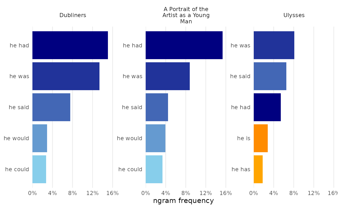
The ignore parameter stipulates values to remove from
the Y-axis to focus a figure.
sentiment_ulysses |>
  visualize(ignore = c("anger", "anticipation", "disgust", "fear", "trust", "positive", "negative"))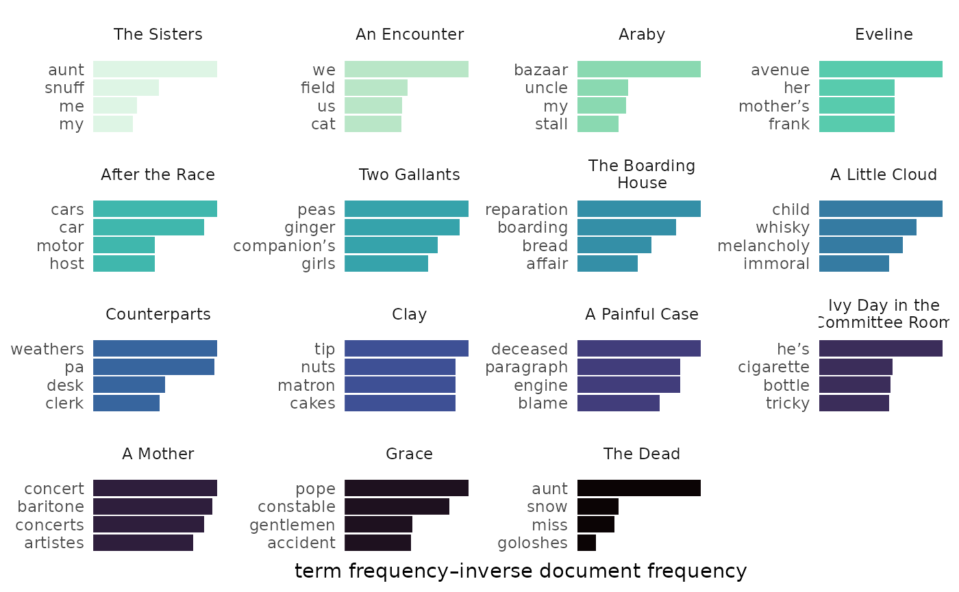
N-grams
For n-grams, visualize() typically returns a network
visualization inspired by the bigram network in Text Mining with
R.
bigrams_joyce |>
  visualize()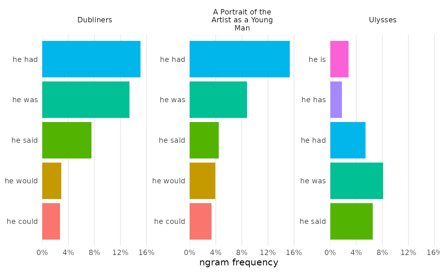
Combining n-grams
N-gram frequencies can be compared by combining them before visualization. Certain arguments allow for deviation from typical charts, including choosing the rows to chart and modifying colors to be set by values on the Y-axis.
bigrams_joyce |>
  dplyr::filter(word_1 == "he") |>
  combine_ngrams() |>
  visualize(rows = 1:5, color_y = TRUE)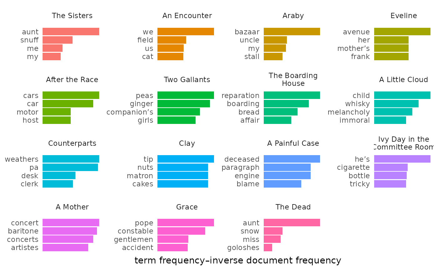
Tf-idf
visualize() returns bars showing the top words for each
document. This can be a useful way to differentiate texts in a set from
each other. Because tfidf_dubliners was prepared with
load_texts(remove_names = TRUE), the resulting chart shows
clearer delineation of topics characteristic of the stories in Joyce’s
collection:
tfidf_dubliners |>
  visualize(rows = 1:4)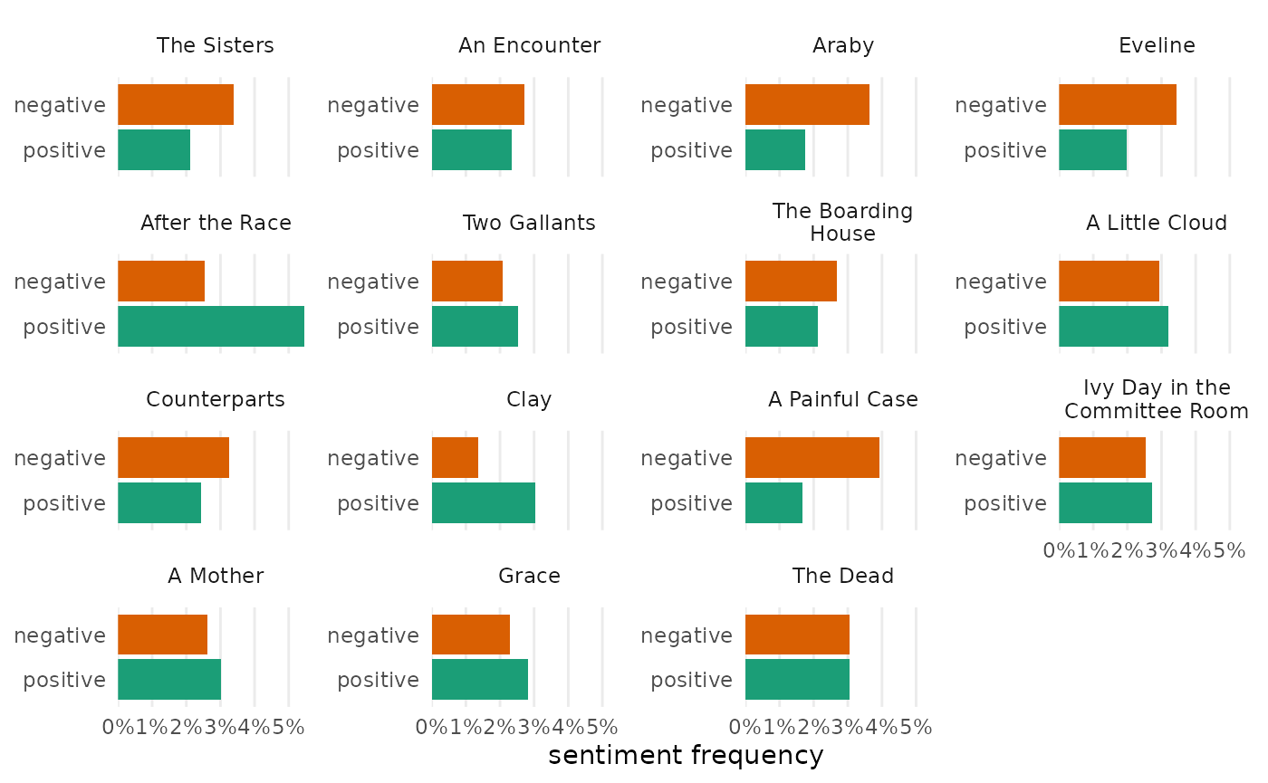
Changing colors
change_colors() does what its name implies. By default,
it adopts the “Dark2” palette from Brewer.
sentiment_dubliners |>
  visualize() |>
  change_colors()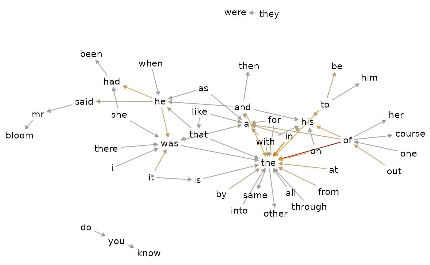
Colors can be chosen manually.
library(ggraph)
bigrams_joyce |>
  visualize(top_n = 60) |>
  change_colors(c("#999999",
                  "orange",
                  "darkred"))
Optionally, use a named vector to set some colors by value instead of by order. By default unnamed colors are gray.
bigrams_joyce |>
  dplyr::filter(word_1 == "he") |>
  combine_ngrams() |>
  visualize(rows = 1:5, color_y = TRUE, reorder_y = TRUE) |>
  change_colors(c(
    "he is" = "darkorange",
    "he has" = "orange"))
Unnamed colors fill in as needed.
bigrams_joyce |>
  dplyr::filter(word_1 == "he") |>
  combine_ngrams() |>
  visualize(rows = 1:5, color_y = TRUE, reorder_y = TRUE) |>
  change_colors(c(
    # Highlight two bars as outliers:
    "he is" = "darkorange",
    "he has" = "orange",
    # Custom gradient palette:
    "midnightblue", "lightseagreen", "mediumspringgreen"
    ))
Or choose a predetermined color set and palette, as described in function documentation.
tfidf_dubliners |>
  visualize(rows = 1:4) |>
  change_colors(colorset = "viridis", palette = "mako", direction = -1)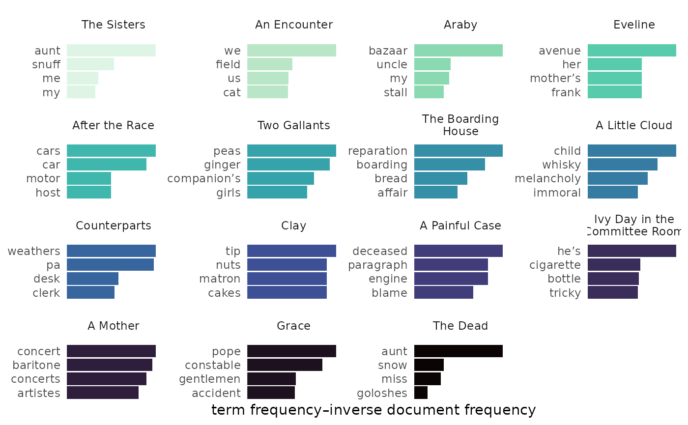
Italicizing titles
Before sharing a figure, italicize_titles() adds one
more step of polish:
bigrams_joyce |>
  combine_ngrams() |>
  visualize(rows = 1:5, color_y = FALSE, reorder_y = TRUE) |>
  italicize_titles()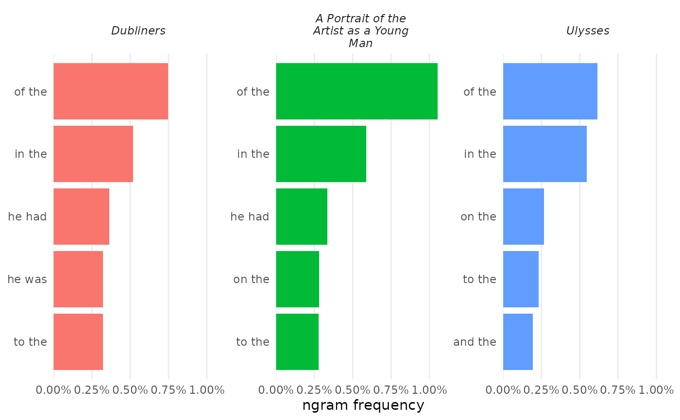
corpus_joyce |>
  visualize() |>
  italicize_titles()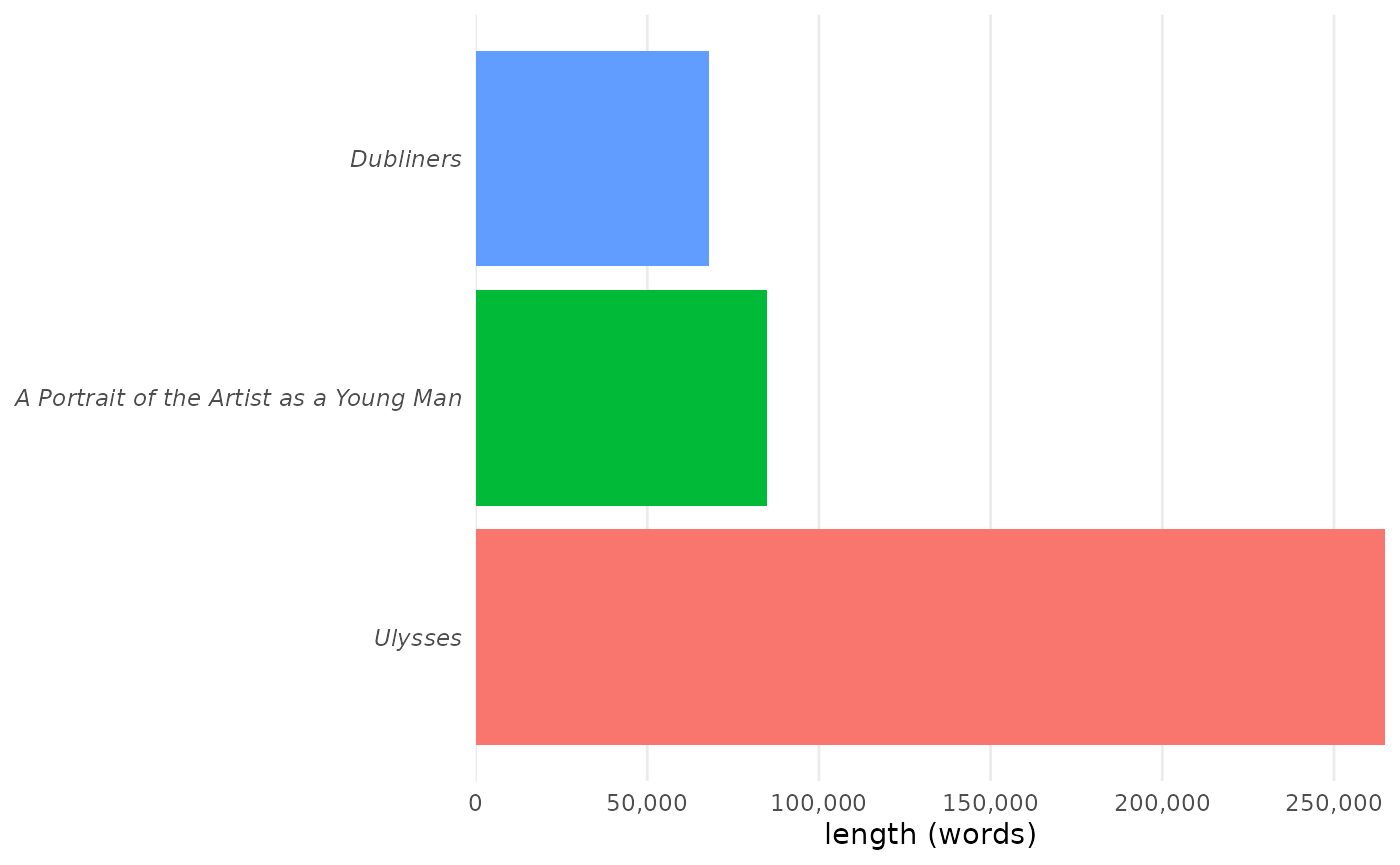
Explaining process
When it’s time to write up the methods used to find a set of
conclusions, it’s important to document the steps taken.
narrativize() helps turn a logged set of steps into bullet
points or a paragraph of methods:
bigrams_joyce |>
  narrativize()
#>  - Retrieved a corpus from Project Gutenberg using ID numbers 2814, 4217, and 4300.
#>  - Moved column `subsection` into body text.
#>  - Loaded texts by tokenizing words, converting to lowercase, and preserving paragraph breaks.
#>  - Identified documents using the column `title`.
#>  - Constructed bigram sequences from the text.
Options allow for changes in format and person, but the final output will still need some manual tweaking.
bigrams_joyce |>
  narrativize(format = "text", person = "we", return = "html")