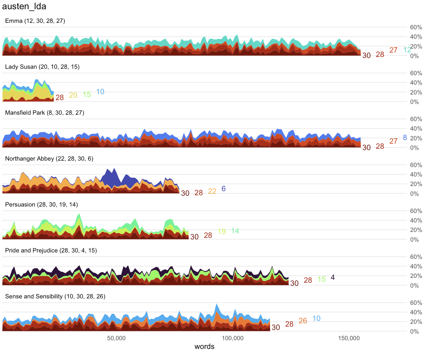
plot_topic_distributions() prepares a visualization for exploring the most significant topics in each document over time.
Usage
plot_topic_distributions(
  lda,
  top_n = 4,
  direct_label = TRUE,
  title = TRUE,
  save = TRUE,
  saveas = "png",
  savedir = "plots",
  omit = NULL,
  smooth = TRUE
)
Arguments
- lda
The topic model to be used.
- top_n
The number of topics to visualize. By default, the top 4 topics in each document will be shown.
- direct_label
By default, directly labels topic numbers on the chart. Set it to FALSE to show a legend corresponding to each color.
- title
By default, the function will add a title to the chart, corresponding to the name of the object passed to the
ldaparameter. Set it to FALSE to return a chart with no title.- save
By default, the visualization will be saved. Set to FALSE to skip saving.
- saveas
The filetype for saving resulting visualizations. By default, the files will be in "png" format, but other options such as "pdf" or "jpg will also work.
- savedir
The directory for saving output images. By default, this is set to "plots/".
- omit
Upon exploration, some topics may be found to contain common stop words or other unhelpful material. Use the
omitparameter to define a vector of topic numbers you wish to omit from a visualization.- smooth
After samples are rejoined, the measured value of each topic will vary wildly, even in samples that are beside each other in a document. This can make charts distractingly jittery. The default TRUE value of this parameter reduces chart noise by calculating rolling averages across three samples. Set the parameter to FALSE to skip this step and allow for visualization of extreme values.
Value
A ggplot2 visualization showing vertical facets of texts. The length of each text is shown on the X-axis, and area plots on the Y-axis show the distribution of the strongest topics in each part of the text.
Examples
austen <-
  get_gutenberg_corpus(c(105, 121, 141, 158, 161, 946, 1342)) |>
  dplyr::select(doc_id = title, text)

austen_lda <-
  austen |>
  make_topic_model(k = 30)

plot_topic_distributions(austen_lda)